Run the analysis
Lorenzo Cattarino
2020-09-15
Source:vignettes/how_to_run_analysis.Rmd
how_to_run_analysis.RmdWe first load the package.
We then need to download the database of global disaggregated FOI and environmental and demographic covariates values at 1/6 decimal degree resolution. This is a data frame with 425138 rows and 43 columns:
my_url <- "https://mrcdata.dide.ic.ac.uk/resources/DENVfoiMap/all_squares_env_var_0_1667_deg.rds"

all_sqr_covariates <- readRDS(url(my_url))
We define some parameters
extra_prms <- list(id_fld = "unique_id",
                   grp_flds = c("unique_id", "ID_0", "ID_1"),
                   ranger_threads = NULL,
                   fit_type = "boot",
                   parallel_2 = FALSE,
                   screening_ages = c(9, 16),
                   target_nm = c("I", "C", "HC", "R0_1", "R0_2"),
                   coord_limits = c(-74, -32, -34, 6))

my_col <- colorRamps::matlab.like(100)
and variables which depend on those parameters.
parameters <- create_parameter_list(extra_params = extra_prms)

all_wgt <- parameters$all_wgt

all_predictors <- predictor_rank$name

base_info <- parameters$base_info

foi_offset <- parameters$foi_offset

coord_limits <- parameters$coord_limits

screening_ages <- parameters$screening_ages
Now we do some preprocessing.
foi_data$new_weight <- all_wgt

pAbs_wgt <- get_sat_area_wgts(foi_data, parameters)

foi_data[foi_data$type == "pseudoAbsence", "new_weight"] <- pAbs_wgt
We create one bootstrap sample of the data.
foi_data_all_bsamples <- grid_and_boot(data_df = foi_data, parms = parameters)

foi_data_bsample <- foi_data_all_bsamples[[1]]
We then fit the random forest model. This takes approximately 20-30 minutes.
RF_obj_optim <- full_routine_bootstrap(parms = parameters,
                                       original_foi_data = foi_data,
                                       adm_covariates = admin_covariates,
                                       all_squares = all_sqr_covariates,
                                       covariates_names = all_predictors,
                                       boot_sample = foi_data_bsample)
We can make force of infection predictions using a dataset of covariates. In this example we will do it for Brazil only to reduce computing time.
BRA_ID_0 <- 33

BRA_sqr_covariates <- all_sqr_covariates[all_sqr_covariates$ID_0 == BRA_ID_0,]

BRA_predictions <- make_ranger_predictions(RF_obj_optim,
                                           dataset = BRA_sqr_covariates,
                                           covariates_names = all_predictors)

BRA_predictions <- BRA_predictions - foi_offset
BRA_predictions[BRA_predictions < 0] <- 0

BRA_sqr_covariates$p_i <- BRA_predictions
And now we make a map of predicted force of infection for Brazil.
# map
map_data_df <- map_preprocess(BRA_sqr_covariates, "p_i", parameters)
q_map <- quick_raster_map(pred_df = map_data_df,
                          my_col = my_col,
                          ttl = "FOI",
                          parms = parameters)
q_map
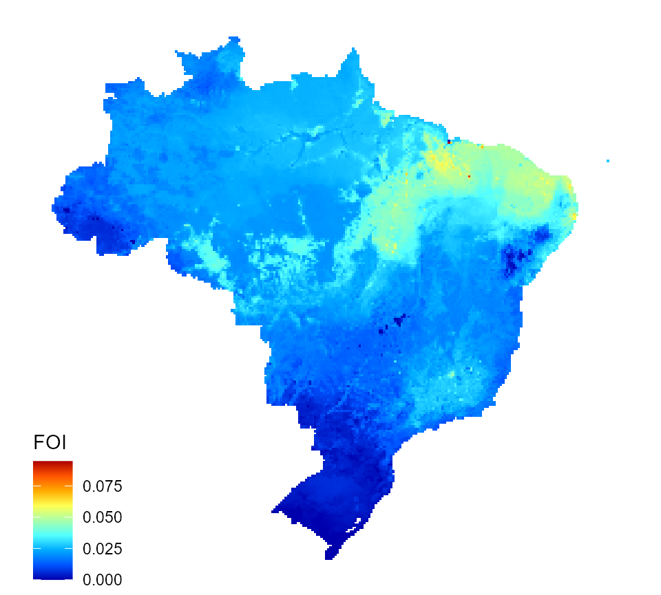
Predicted dengue force of infection for Brazil
We can now calculate the dengue reproduction number, \(R_{0}\), corresponding to the predicted force of infections, and the burden estimates. We can use the drep package for this.
# preprocessing
age_band_tgs <- grep("band", names(age_structure), value = TRUE)
age_band_bnds <- drep::get_age_band_bounds(age_band_tgs)
age_band_L_bounds <- age_band_bnds[, 1]
age_band_U_bounds <- age_band_bnds[, 2]

# create lookup tables - this takes 5-10 minutes
lookup_tabs <- create_lookup_tables(
  age_struct = age_structure,
  age_band_tags = age_band_tgs,
  age_band_L_bounds = age_band_L_bounds,
  age_band_U_bounds = age_band_U_bounds,
  parms = parameters)

# assume a transmission reduction effect of 0% (scale factor = 1)
sf_val <- parameters$sf_vals[1]

# attach look up table id
sqr_preds_2 <- dplyr::inner_join(age_structure[, c("age_id", "ID_0")],
                                 BRA_sqr_covariates,
                                 by = "ID_0")

sqr_preds_3 <- as.matrix(sqr_preds_2)

burden_estimates_raw <- wrapper_to_replicate_R0_and_burden(
  foi_data = sqr_preds_3,
  scaling_factor = sf_val,
  FOI_to_Inf_list = lookup_tabs[[1]],
  FOI_to_C_list = lookup_tabs[[2]],
  FOI_to_HC_list = lookup_tabs[[3]],
  FOI_to_R0_1_list = lookup_tabs[[4]],
  FOI_to_R0_2_list = lookup_tabs[[5]],
  parms = parameters)

burden_estimates <- post_processing_burden(sqr_preds_3, burden_estimates_raw, parameters)
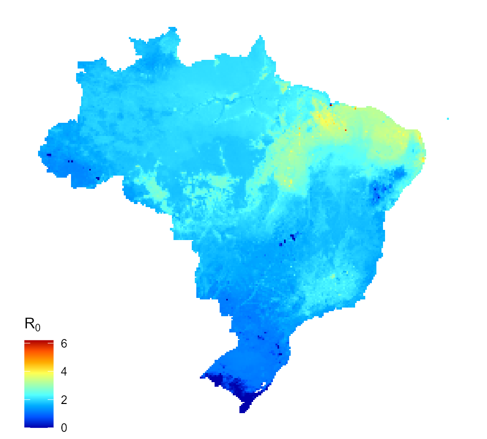
We can map one \(R_{0}\), for instance the one for assumption 1, only primary and secondary infections are infectious.
map_data_df <- map_preprocess(burden_estimates, "transformed_1", parameters)
r0_map_1 <- quick_raster_map(pred_df = map_data_df,
                             my_col = my_col,
                             ttl = expression("R"[0]),
                             parms = parameters)
r0_map_1

Predicted dengue reproduction number for Brazil (assumption 1)
Or the \(R_{0}\) for assumption 2, all infections (primary to quaternary) are infectious.
map_data_df <- map_preprocess(burden_estimates, "transformed_2", parameters)
r0_map_2 <- quick_raster_map(pred_df = map_data_df,
                             my_col = my_col,
                             ttl = expression("R"[0]),
                             parms = parameters)
r0_map_2
Predicted dengue reproduction number for Brazil (assumption 2)
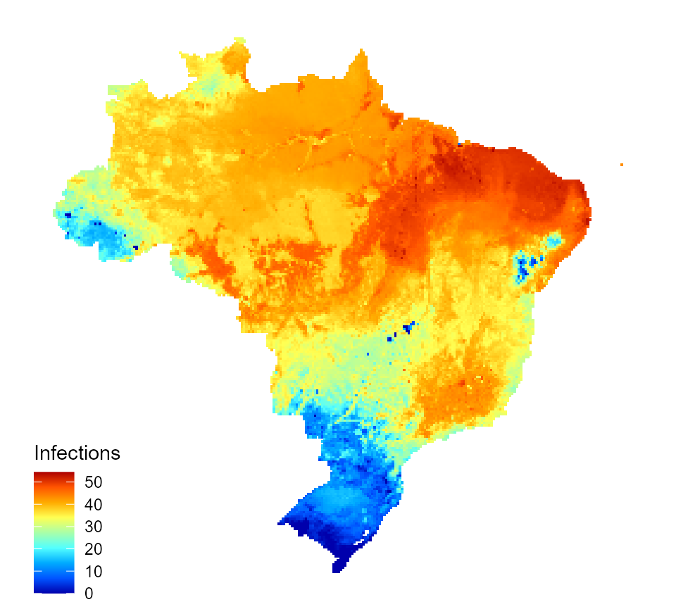
We can also map a burden measure, e.g. the incidence of annual infections (per 1000).
burden_estimates$I_num_inc <- burden_estimates$I_num / burden_estimates$population * 1000

map_data_df <- map_preprocess(burden_estimates, "I_num_inc", parameters)
inc_inf_map <- quick_raster_map(pred_df = map_data_df,
                                my_col = my_col,
                                ttl = "Infections",
                                parms = parameters)
inc_inf_map
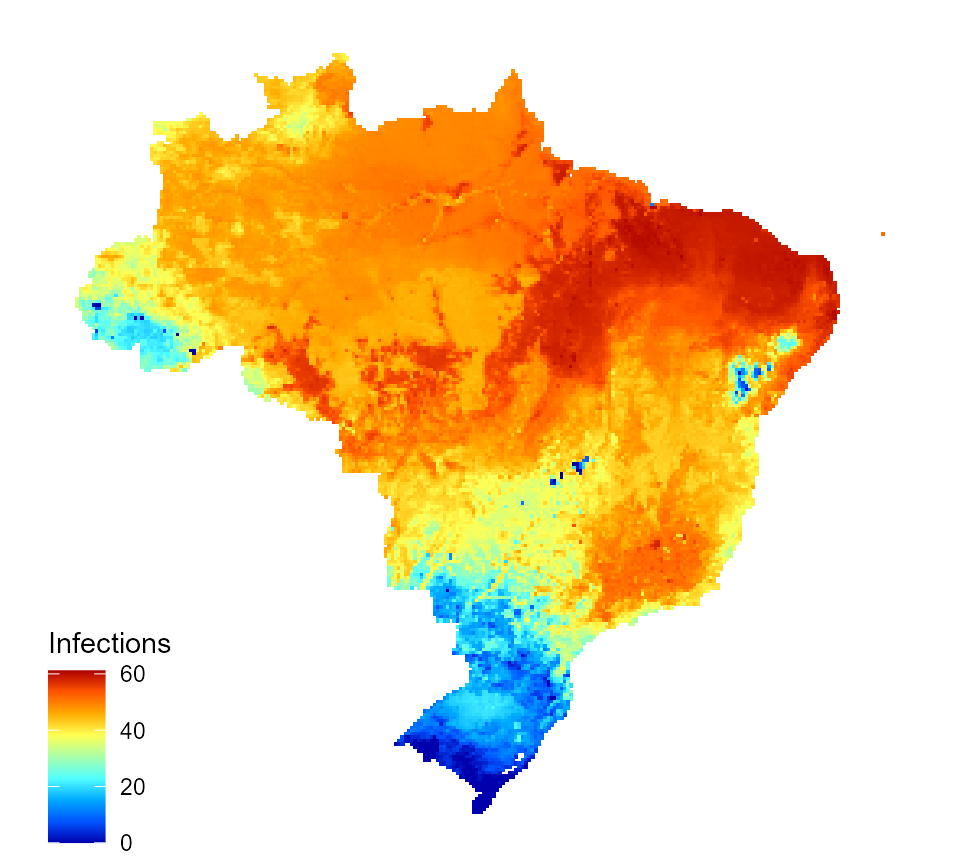
Predicted incidence of annual dengue infections for Brazil
We now estimate the impact of control strategies using the predicted \(R_{0}\). We first look at a transmission-reduction type of intervention, such as Wolbachia).
# assume a transmission reduction effect of 30%
sf_val <- parameters$sf_vals[4]

tr_red_impact_estimates_raw <- wrapper_to_replicate_R0_and_burden(
  foi_data = sqr_preds_3,
  scaling_factor = sf_val,
  FOI_to_Inf_list = lookup_tabs[[1]],
  FOI_to_C_list = lookup_tabs[[2]],
  FOI_to_HC_list = lookup_tabs[[3]],
  FOI_to_R0_1_list = lookup_tabs[[4]],
  FOI_to_R0_2_list = lookup_tabs[[5]],
  parms = parameters)

tr_red_impact_estimates <- post_processing_burden(sqr_preds_3, tr_red_impact_estimates_raw, parameters)
And then map the incidence of infections following the intervention (for \(R_{0}\) assumption 1).
tr_red_impact_estimates$I_num_1_inc <- tr_red_impact_estimates$I_num_1 / tr_red_impact_estimates$population * 1000
mp_nm <- "Infections_30pc_tr_red_impact.png"
map_data_df <- map_preprocess(tr_red_impact_estimates, "I_num_1_inc", parameters)
inc_inf_map_30pc_tr <- quick_raster_map(pred_df = map_data_df,
                                        my_col = my_col,
                                        ttl = "Infections",
                                        parms = parameters)
inc_inf_map_30pc_tr
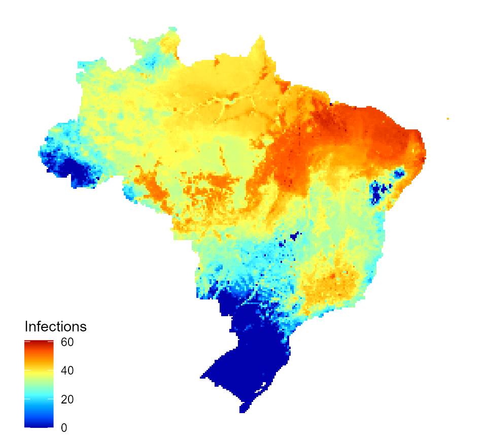
Predicted incidence of annual dengue infections for Brazil following application of an intervention with 30% transmission reduction effect
Finally, we predict the impact of the Sanofi-Pasteur dengue vaccine using estimates of the vaccine effect size from this study and our \(R_{0}\) predictions (assumption 1 in this example).
R0_1_preds <- burden_estimates$transformed_1

my_look_up_table <- pre_process_vaccine_lookup_table(R0_to_prop_infections_averted_lookup_1, R0_1_preds)

screen_age <- screening_ages[1] # 9 years olds

prop_averted <- approx(my_look_up_table[, "R0"], my_look_up_table[, screen_age], xout = R0_1_preds)$y

burden_net_vaccine <- (1 - prop_averted) * burden_estimates[, "I_num"]

burden_estimates_2 <- cbind(burden_estimates[, base_info], I_vacc_impact = burden_net_vaccine)
We map incidence of infections following vaccination.
burden_estimates_2$I_num_1_inc_v <- burden_estimates_2$I_vacc_impact / burden_estimates_2$population * 1000

map_data_df <- map_preprocess(burden_estimates_2, "I_num_1_inc_v", parameters)
inc_inf_map_vacc <- quick_raster_map(pred_df = map_data_df,
                                     my_col = my_col,
                                     ttl = "Infections",
                                     parms = parameters)
inc_inf_map_vacc
Predicted incidence of annual dengue infections for Brazil following vaccination of 9 years olds (80% vaccine coverage)